INTRODUCTION
In today’s digital age, online shopping has transformed consumer behavior. With the click of a button, shoppers can access a plethora of products, and their purchasing decisions are often influenced by product reviews and ratings available on e-commerce platforms. These platforms, especially in the realm of clothing and fashion, amass a vast volume of customer feedback. Delving into these reviews can unearth insights into customer sentiments, preferences, and overall product perception.
OBJECTIVE
The primary objective of this analysis is to dissect e-commerce clothing reviews to glean meaningful insights. By understanding customer sentiments, pinpointing standout products or features, and discerning patterns or trends in feedback, e-commerce businesses can harness these insights to enhance product offerings, fine-tune marketing strategies, and ultimately elevate customer satisfaction.
DATASET INFORMATION
This analysis is anchored on a dataset encompassing e-commerce clothing reviews. The dataset includes 23486 rows and 10 feature variables. Each row corresponds to a customer review, and includes the variables: offering a holistic view into customer feedback, and incorporating the following key attributes:
- Review Text: The narrative content shared by the customer.
- Rating: A score, typically ranging from 1 to 5, conferred by the customer to the product.
- Division Name: Specifies the division to which the reviewed product is categorized.
- Department Name: Indicates the overarching department under which the product resides.
- Class Name: Details the specific category or class of the clothing item reviewed.
- Age: Sheds light on the age bracket of the reviewer.
- Clothing ID: A unique identifier associated with each clothing item.
- Title: A concise title or headline for the review, capturing its essence.
- Recommended IND: A binary indicator reflecting whether the product garners a recommendation from the reviewer (1 indicating “Yes”, and 0 indicating “No”).
- Positive Feedback Count: Quantifies the number of positive feedbacks a particular review has accumulated.
While the primary exploration revolves around the aforementioned columns, some dataset might also harbor other auxiliary details that can be tapped into, depending on the scope of the analysis.”
IMPORTING NECESSARY LIBRARIES
Before diving into the analysis, it’s essential to equip ourselves with the right tools. In the realm of Python-based data analysis, several libraries stand out as indispensable:
NumPy: Renowned for its capabilities in numerical computing, NumPy provides an array of tools for working with high-performance arrays and matrices. Its efficient mathematical functions underpin many data operations.
Pandas (pd): An invaluable resource for data manipulation and analysis, Pandas offers data structures like DataFrames that make handling and processing structured data seamless.
Matplotlib (plt) and Seaborn (sns): When it comes to visualizing data, these two libraries are the dynamic duo. Matplotlib provides a broad spectrum of plotting tools, while Seaborn, built on top of Matplotlib, offers a higher-level interface for creating aesthetically pleasing and informative statistical graphics.
TextBlob: In the world of natural language processing, TextBlob emerges as a simple API for delving into common text processing tasks. For this analysis, it’s pivotal in assessing the sentiment of the reviews.
CountVectorizer from sklearn.feature_extraction.text: This tool from the Scikit-learn library assists in converting a collection of text documents into a matrix of token counts. It’s a foundational step when transforming text data for machine learning algorithms.
Lastly, to ensure a smooth and uninterrupted analysis experience, any warnings generated during code execution are silenced using the warnings module.
import numpy as np import pandas as pd import matplotlib.pyplot as plt import seaborn as snspip install wordcloud from wordcloud import WordCloud, STOPWORDSfrom textblob import TextBlob from sklearn.feature_extraction.text import CountVectorizer import warnings warnings.filterwarnings('ignore')
Having installed these libraries and tools, we’re ready to conduct a comprehensive and insightful analysis of the e-commerce clothing reviews.
Importing the Dataset
To kickstart our analysis, the first step involves importing the dataset into our Python environment. This is achieved using the read_csv() function from the Pandas library, a powerful tool tailored for reading structured data files. Once loaded, we display the first five rows of the dataset using the head() method. This initial glimpse offers a snapshot of the dataset’s structure and the kind of data we’ll be working with:
df = pd.read_csv('data.csv')
df.head()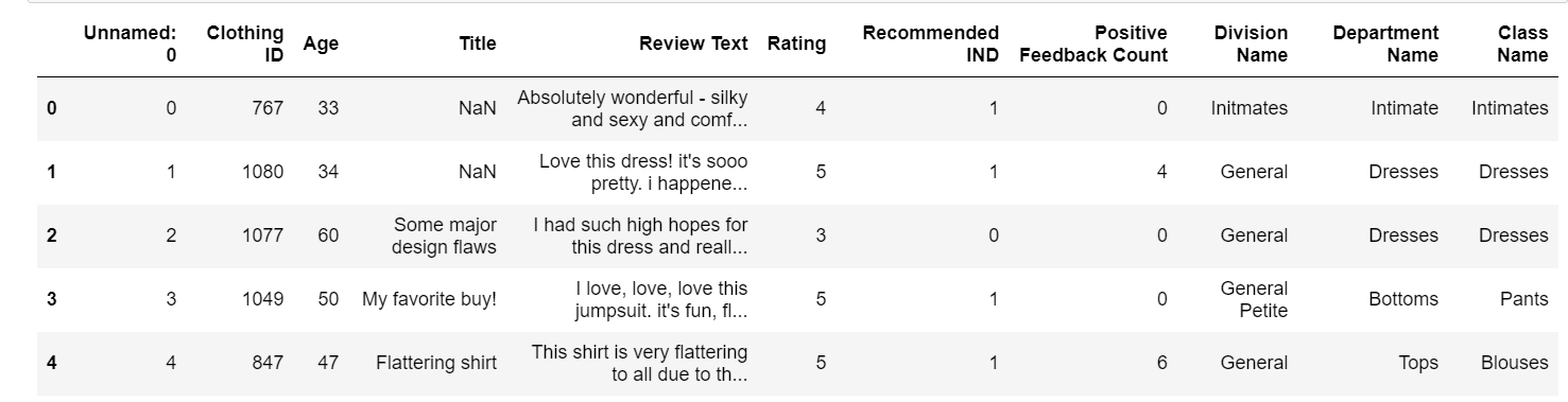
Data Preprocessing
Before delving into the analysis, it’s important to ensure the integrity and quality of our dataset. The preprocessing phase addresses potential discrepancies and prepares the data for in-depth exploration.
Data Cleaning: Data cleaning is foundational to any analytical project. It involves identifying and rectifying (or omitting) errors and inconsistencies. The importance of this step cannot be overstated, as flawed or inconsistent data can skew results or spawn misleading interpretations.
Handling Missing Values: The completeness of data is paramount. An initial assessment spotlighted missing values across various columns.
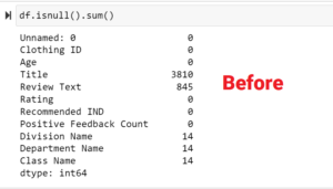
As a corrective measure:
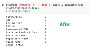
- Specific columns, notably ‘Unnamed: 0’ and ‘Title’, were excised.
- Rows marred by missing values were purged to guarantee a consistent dataset.
Text Preprocessing: The ‘Review Text’ column, central to our dataset with its customer reviews, was subjected to rigorous preprocessing to enhance its clarity and standardization:
- HTML Tags Removal: Residual HTML tags, exemplified by
<br/>, were eliminated, preserving the human-centric essence of the reviews. - Hyperlink Extraction: Hyperlinks, generally ensconced within
<a></a>tags, were identified and expunged. - Special Character Rectification: Special characters and entities, such as
&,>, and<, were addressed and eradicated. In addition, non-breaking space characters (\\xa0) were supplanted with conventional space characters.
def preprocess(ReviewText):
ReviewText = ReviewText.str.replace("(<br/>)", "")
ReviewText = ReviewText.str.replace('(<a).*(>).*(</a>)', '')
ReviewText = ReviewText.str.replace('(&)', '')
ReviewText = ReviewText.str.replace('(>)', '')
ReviewText = ReviewText.str.replace('(<)', '')
ReviewText = ReviewText.str.replace('(\xa0)', ' ')
return ReviewText
df['Review Text'] = preprocess(df['Review Text'])Through assiduous preprocessing, especially of the review text, the stage is set for an analysis rooted in clean, standardized, and significant data.
FEATURE ENGINEERING
Feature engineering is a subset of data preprocessing. This involves creating new features (columns) from the existing data to improve the dataset’s utility for modeling or analysis. We’re enhancing our dataset by adding three new columns: ‘Polarity’, ‘word_count’, and ‘review_len’.
- Polarity: Using TextBlob, we assess the sentiment of each review. This gives us a score between -1 and 1 — where 1 indicates a positive sentiment, -1 indicates a negative sentiment, and values around 0 are neutral.
- word_count: This column shows how many words are in each review. It’s calculated by splitting the review text into individual words and counting them.
- review_len: Here, we’re counting the total number of characters in each review, giving us an idea of its length.
These additions will help us gain deeper insights into the reviews and their characteristics.
df['Polarity'] = df['Review Text'].apply(lambda x: TextBlob(x).sentiment.polarity)
df['word_count'] = df['Review Text'].apply(lambda x: len(str(x).split()))
df['review_len'] = df['Review Text'].apply(lambda x: len(str(x)))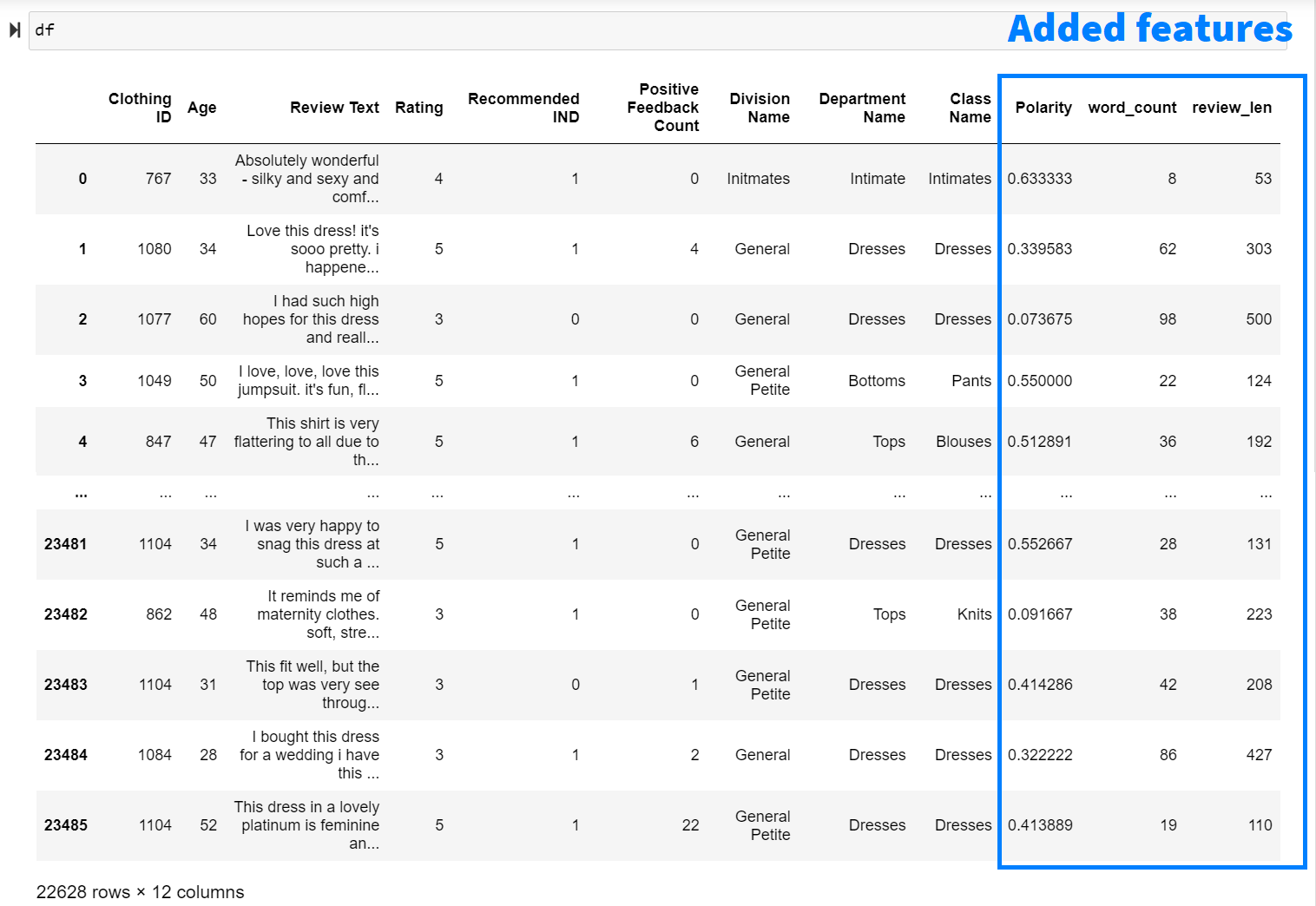
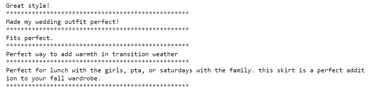
To understand the different details of the reviews’ sentiments, we’ll delve into a few representative examples across different sentiment ranges. We’ll begin by exploring reviews that are entirely positive, bearing a sentiment polarity of 1. Subsequently, we’ll pivot to reviews that are neutral, with a polarity score of 0, suggesting an absence of discernible sentiment. Lastly, we’ll spotlight some of the strongly negative reviews, those with a polarity less than or equal to -0.7. These reviews likely contain pronounced negative feedback or criticism. Displaying these samples will provide a tangible sense of the sentiments present in our dataset, from the glowing commendations to the more critical evaluations.
Polarity == 1 (Positive reviews)
cl = df.loc[df.Polarity == 1, ['Review Text']].sample(5).values
for c in cl:
    print(c[0])
    print("**************************************************")
Polarity == 0 (Neutral Reviews)
cl = df.loc[df.Polarity == 0, ['Review Text']].sample(5).values
for c in cl:
    print(c[0])
    print("**************************************************")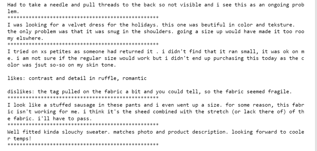
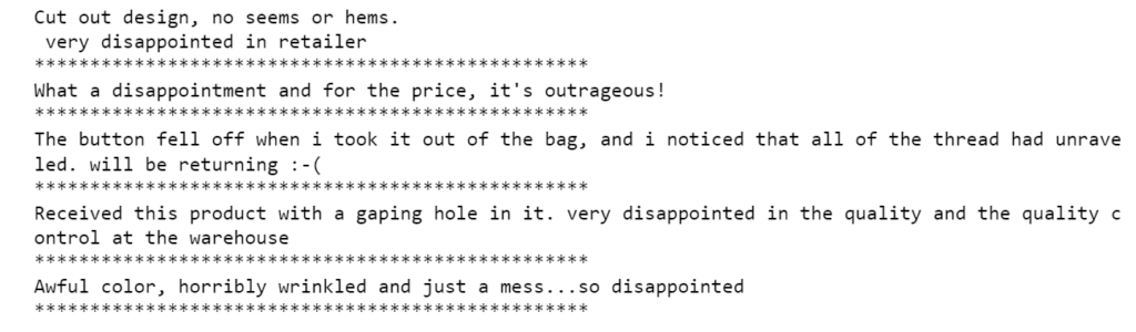
Polarity <= – 0.7
cl = df.loc[df.Polarity <= -0.7, ['Review Text']].sample(5).values
for c in cl:
    print(c[0])
    print("**************************************************")
DATA VISUALIZATION
To gain a deeper understanding of our dataset’s characteristics, we’ll visualize the distributions of several key features: ‘Polarity’, ‘Age’, ‘review_len’, and ‘word_count’. We begin by defining a list of these features alongside corresponding titles for our plots and preferred colors for each histogram. Leveraging the Seaborn library, we iterate over these lists and employ the sns.distplot() function to craft a series of histograms. Each histogram provides a granular view of how data points are spread across different ranges for a given feature. For instance, the ‘Polarity Distribution’ will show us the spread of sentiment scores, while the ‘Age Distribution’ will reveal the age demographics of our reviewers.
features = ['Polarity', 'Age', 'review_len', 'word_count']
titles = ['Polarity Distribution', 'Age Distribution', 'Review length Distribution', 'Word Count Distribution']
colors = ['#9966ff', '#3399ff', '#00ff00', '#ff6600']

for feature, title, color in zip(features, titles, colors):
    sns.distplot(x=df[feature], bins=50, color=color)
    plt.title(title, size=15)
    plt.xlabel(feature)
    plt.show()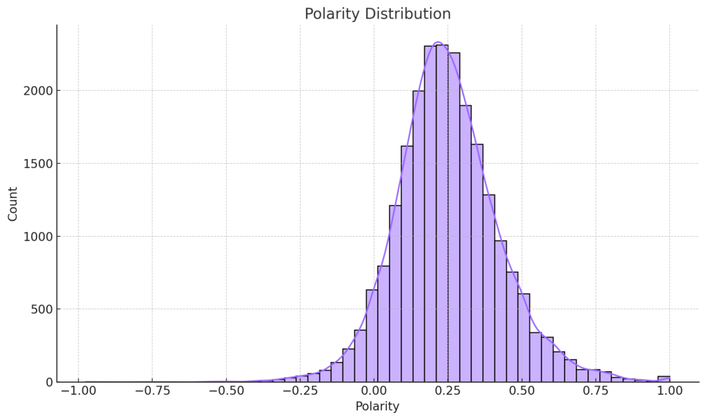
Polarity Distribution: This histogram showcases the spread of sentiment scores in the dataset. The majority of reviews have a positive polarity, indicating that most customers had favorable experiences. However, there’s a considerable amount of reviews around the neutral zone (close to 0), and a smaller portion of reviews are negative.
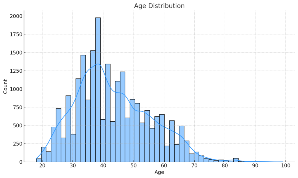
Age Distribution: This plot provides insight into the age demographics of the reviewers. It seems that the majority of reviews are written by individuals in their 30s to 50s.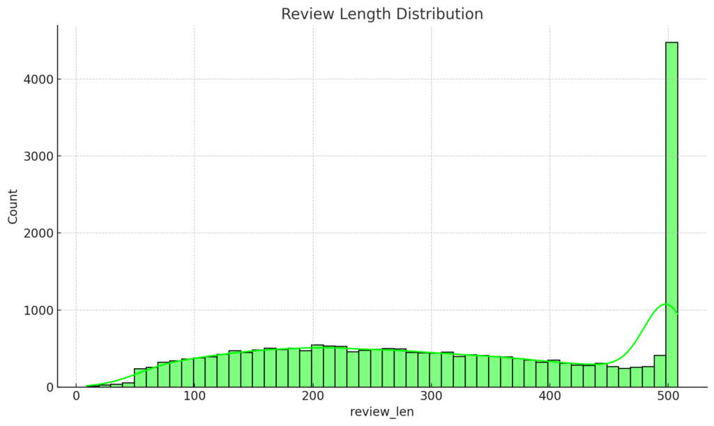
Review Length Distribution: The majority of reviews are relatively short, with most of them being under 500 characters. However, there are some longer reviews that exceed 1000 characters.
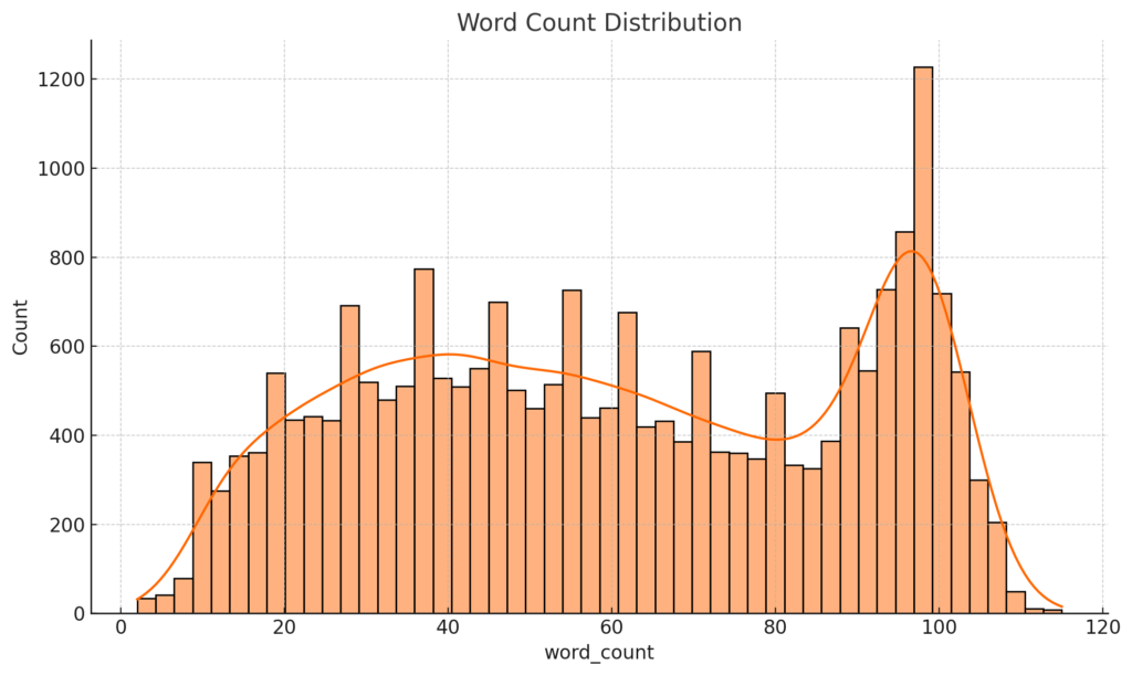
Word Count Distribution: This histogram aligns with the review length distribution. Most reviews are concise, with word counts under 100. However, there are a few reviews that are more verbose, containing more than 200 words.
RATING DISTRIBUTION
The Rating Distribution plot provides a clear picture of the spread of ratings in the dataset
sns.countplot(x = 'Rating', palette='viridis', data=df)
plt.title('Rating Distribution', size=15)
plt.xlabel('Ratings')
plt.show()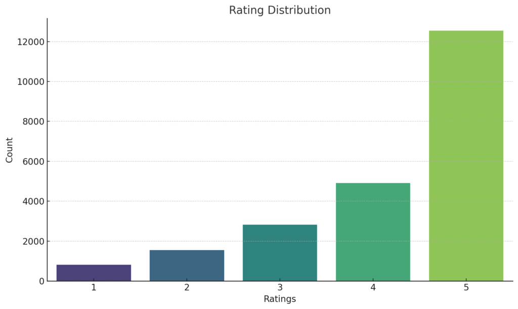
The dominance of high ratings (4 and 5) in the dataset highlights the overall positive sentiment of the reviews. This observation is consistent with the Polarity Distribution, where we noted a significant number of reviews having positive polarity scores. The convergence of these two insights underscores the general satisfaction of customers and aligns with the notion that most of the reviews are affirmative in nature.
Division Distribution
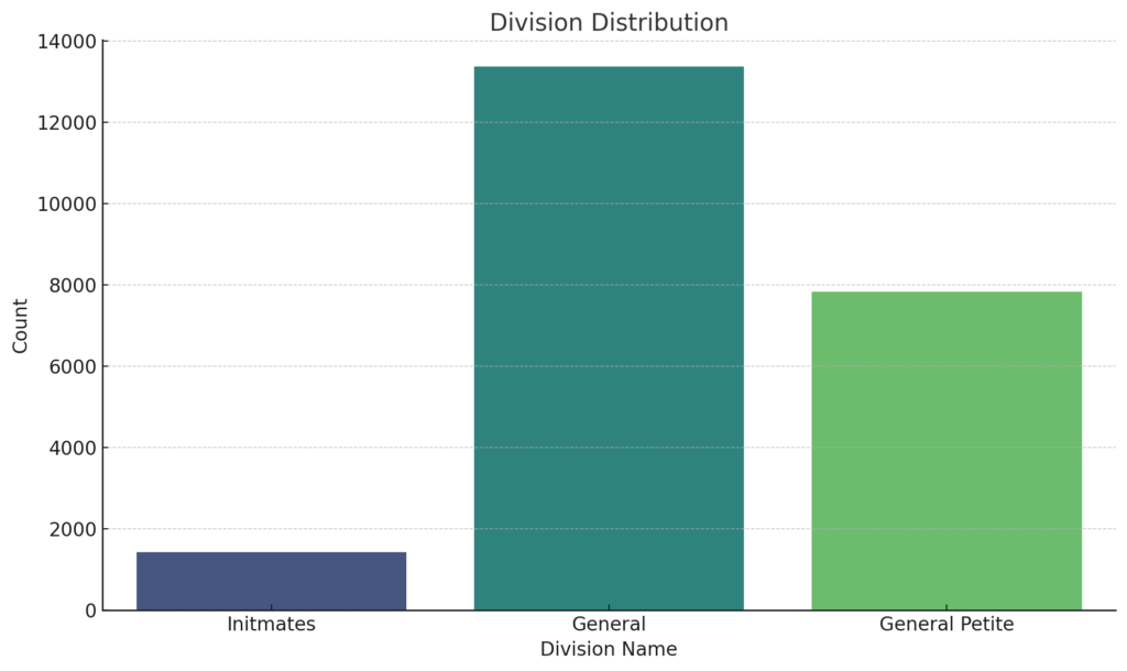
The Division Distribution plot reveals that the “General” division garners the most reviews, suggesting its broad product range resonates with a vast customer base. Meanwhile, the “General Petite” division, which tailors products for petite sizes, also commands a substantial share of reviews, hinting at a dedicated customer segment. In contrast, the “Intimates” division, with the least reviews, might represent a more niche category or possibly a limited product lineup.
Department Distribution
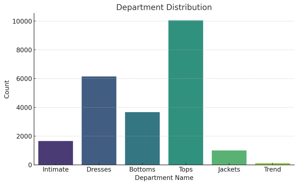
From this distribution, it’s evident that “Tops” and “Dresses” are the most popular and reviewed categories, providing insights into the primary product preferences of customers on this platform.
Class Distribution
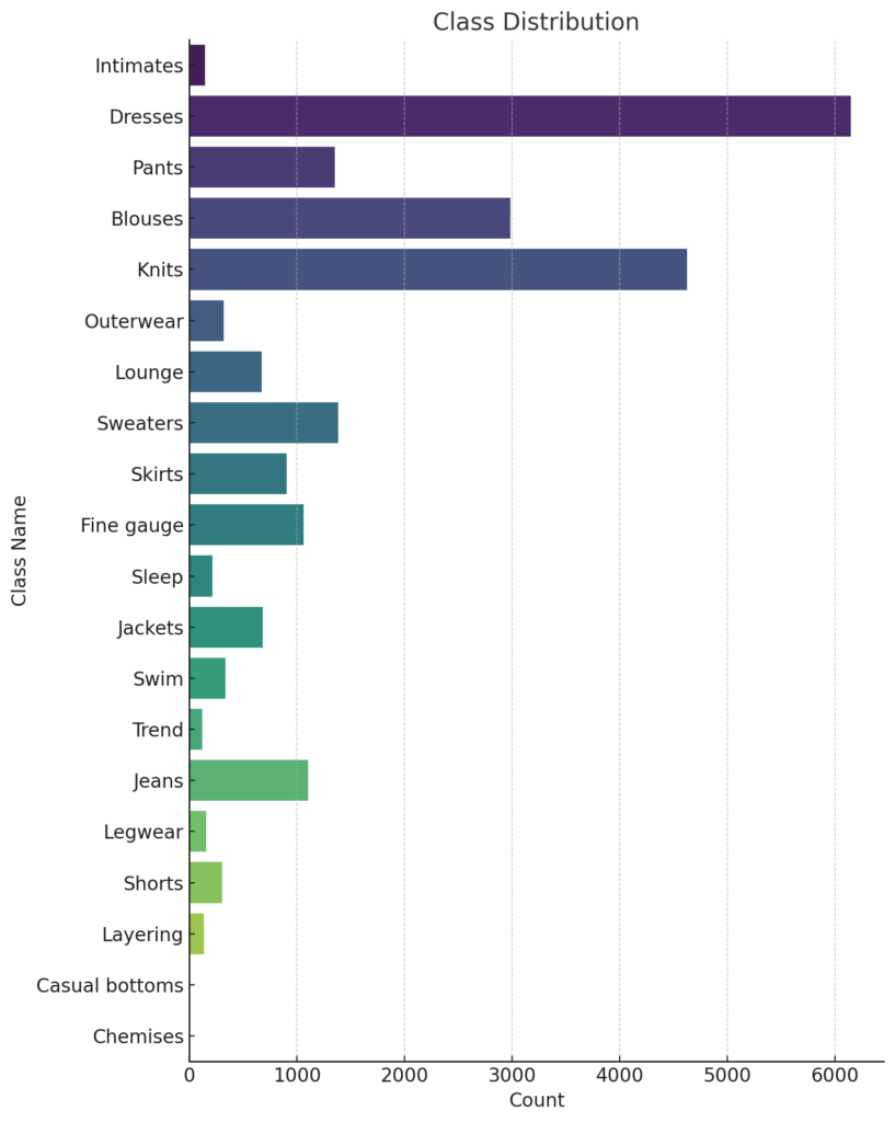
The Class Distribution showcases distinct trends in customer preferences. “Dresses” and “Knits” emerge as the most favored, evidenced by their dominating review volume. Following closely are “Blouses”, “Sweaters”, and “Pants”, which also receive substantial attention from buyers. In contrast, niche classes like “Chemises”, “Casual bottoms”, and “Wedding” have limited reviews, hinting at their specialized nature or potentially limited product offerings in these categories.
N-GRAM ANALYSIS
N-gram analysis is a fundamental concept in natural language processing and text analytics. An N-gram is a contiguous sequence of items from a given sample of text or speech. Depending on the value of , it can take different names:
- Unigram: When , it’s a unigram. It represents a single word. For example, in the sentence “I love ice cream”, the unigrams are “I”, “love”, “ice”, and “cream”.
- Bigram: When , it’s a bigram. It represents a sequence of 2 consecutive words. Using the previous sentence as an example, the bigrams are “I love”, “love ice”, and “ice cream”.
- Trigram: For , it’s called a trigram, representing a sequence of 3 consecutive words. In our example, the trigrams would be “I love ice” and “love ice cream”.
N-gram analysis is crucial for understanding word patterns and relationships within a text, and it’s commonly used in various applications such as text generation, sentiment analysis, and more.
In the realm of N-gram analysis, it’s often essential to consider the removal of stop words. Stop words are common words, such as ‘and’, ‘the’, ‘is’, and others, that, while crucial for sentence construction, often don’t carry significant meaning on their own. When analyzing text for patterns or sentiments, these words can introduce noise, overshadowing more meaningful word combinations. By eliminating these stop words, we refine our N-gram results, spotlighting sequences that genuinely reflect the themes and sentiments present in the text. This refined analysis can lead to more insightful and accurate interpretations. The code block below retrieves the unigram, bigram and trigram from ‘Review Text’ column of the dataframe
def get_top_ngrams(corpus, ngram_range, stop_words=None, n=None):
    vec = CountVectorizer(stop_words=stop_words, ngram_range=ngram_range).fit(corpus)
    bag_of_words = vec.transform(corpus)

    sum_words = bag_of_words.sum(axis=0)

    words_freq = [(word, sum_words[0, idx]) for word, idx in vec.vocabulary_.items()]
    words_freq = sorted(words_freq, key=lambda x: x[1], reverse=True)

    common_words = words_freq[:n]
    words = []
    freqs = []
    for word, freq in common_words:
        words.append(word)
        freqs.append(freq)

    df = pd.DataFrame({'Word': words, 'Freq': freqs})
    return df

stop_words = 'english'
n = 20
unigrams = get_top_ngrams(df['Review Text'], (1, 1), stop_words, n)
bigrams = get_top_ngrams(df['Review Text'], (2, 2), stop_words, n)
trigrams = get_top_ngrams(df['Review Text'], (3, 3), stop_words, n)
UNIGRAMS AND WORDCLOUDS
Unigram and word cloud visualizations are crucial in quickly identifying the main themes or topics in a dataset. By showing the most frequent words, they highlight the dominant sentiments or emotions, like “love” or “disappointed.” These visual tools are essential during initial data exploration, offering an immediate understanding of the text’s essence.
# Plotting
colors = ['#9966ff', '#3399ff', '#00ff00', '#ff6600']
plt.figure(figsize=(8, 10))
sns.barplot(x='Freq', y='Word', color=colors[0], data=unigrams_st)
plt.title('Top 10 Unigrams', size=15)
plt.show()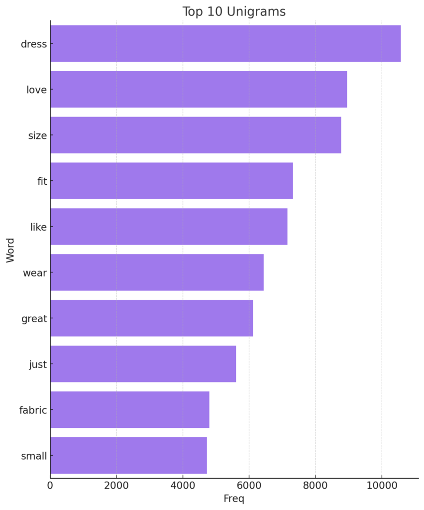
# Generate the word cloud
def generate_wordcloud(text):
    wordcloud = WordCloud(background_color='white',
                          stopwords=STOPWORDS,
                          max_words=200,
                          max_font_size=100,
                          random_state=42,
                          width=800,
                          height=400).generate(text)

    plt.figure(figsize=(12, 6))
    plt.imshow(wordcloud, interpolation='bilinear')
    plt.axis('off')
    plt.show()

# Create a concatenated text from the 'Review Text' column
text = " ".join(review for review in df['Review Text'].astype(str))

# Display the word cloud
generate_wordcloud(text)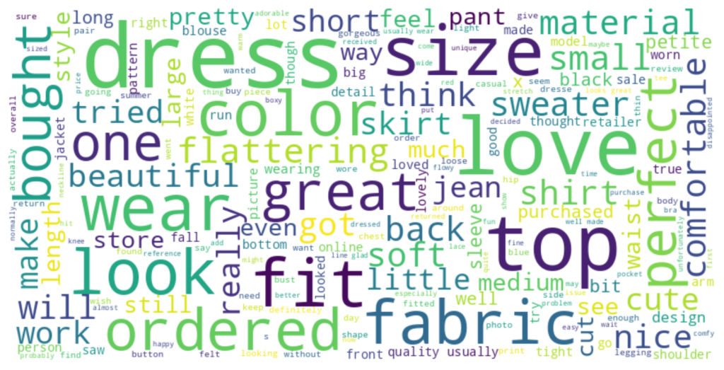
From the two visualizations above, you can observe that words like “love”, “fit”, “dress”, “size”, and “wear” are among the most commonly used words in the reviews, indicating their significance in the feedback provided by customers.
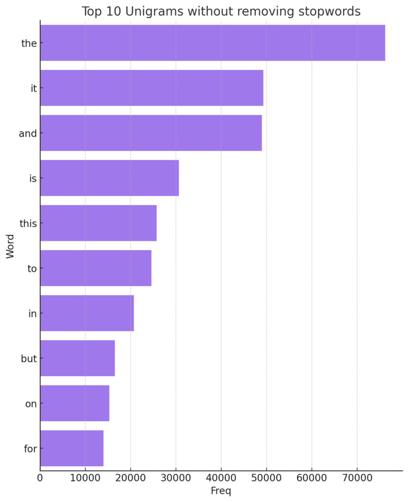
UNIGRAM WITHOUT REMOVING STOP WORDS
Below is the visualization for the top 10 unigrams without removing stopwords. As expected, common words like “the”, “and”, “I”, etc. dominate the chart since stopwords haven’t been filtered out. This demonstrates the importance of removing stopwords when analyzing text data, as they can overshadow the more meaningful words in the content.
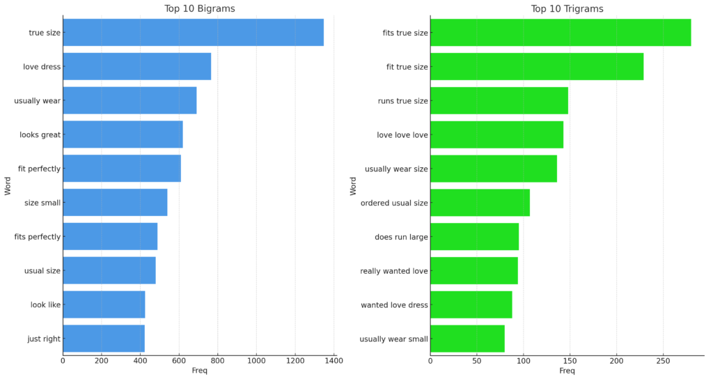
BIGRAMS AND TRIGRAMS
The visualizations below reveal the most frequent bigrams and trigrams in the review texts, emphasizing the importance of fit and size. Bigrams like “fit perfectly” and “true size” indicate positive feedback, while “wanted love” signals unmet expectations. In the trigrams, sequences such as “fit true size” and “looks great fits” provide deeper insights into customer satisfaction, focusing on aesthetics and fit. These n-grams offer e-commerce platforms a lens to pinpoint common praises or criticisms in their reviews, guiding them to either address issues or build on their strengths.
Comparative Analysis by Department
These insights provide a granular look at customer feedback dynamics across different departments, enabling businesses to understand specific areas of strength and potential improvement. Boxplots are particularly apt for this type of analysis as they succinctly represent the distribution of data, highlighting medians, quartiles, and outliers. This allows for a clear comparison of feedback dynamics across departments, emphasizing both general trends and specific deviations.
Sentiment Polarity vs. Department Name:
# Sentiment Polarity v/s Department Name
plt.figure(figsize=(10, 6))
sns.boxplot(x='Department Name', y='Polarity', width=0.5, palette='viridis', data=df)
plt.title('Sentiment Polarity v/s Department Name', size=15)
plt.show()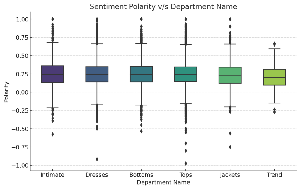
From the visualization, it’s evident that the ‘Trend’ department tends to have a broader range of sentiments, with both high positive and some negative polarities. However, its median sentiment is relatively positive. ‘Intimate’ and ‘Bottoms’ departments exhibit more consistent positive sentiment, with tighter interquartile ranges. Meanwhile, ‘Jackets’ and ‘Tops’ departments showcase a generally positive sentiment but with occasional outliers towards the negative side.
Rating vs. Department Name:
# Rating v/s Department Name
plt.figure(figsize=(10, 6))
sns.boxplot(x='Department Name', y='Rating', width=0.5, palette='viridis', data=df)
plt.title('Rating v/s Department Name', size=15)
plt.show()
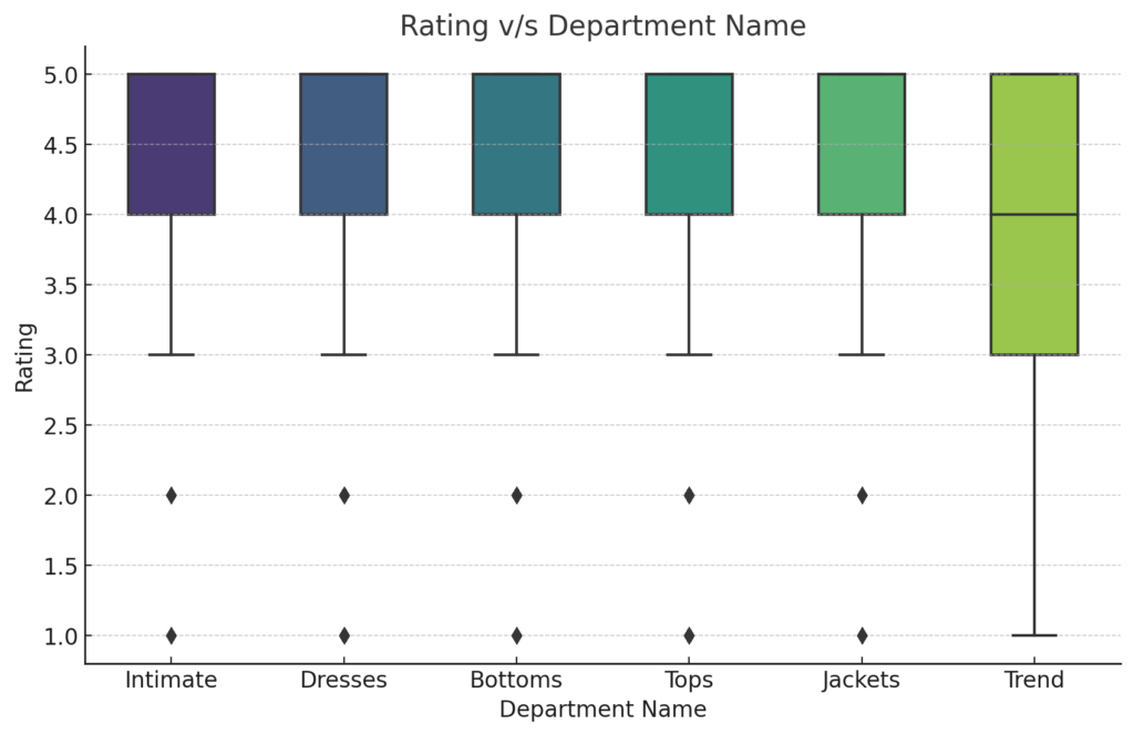
The rating visualization showcases that most departments have a median rating of 4 or above, indicating a generally positive reception among customers. The ‘Intimate’ department stands out with a slightly higher median rating, hinting at higher satisfaction levels for those products. On the other hand, the ‘Trend’ department, despite its positive sentiment polarity, has a wider range in ratings, suggesting more varied customer experiences.
Review Length vs. Department Name:
# Review length v/s Department Name
plt.figure(figsize=(10, 6))
sns.boxplot(x='Department Name', y='review_len', width=0.5, palette='viridis', data=df)
plt.title('Review length v/s Department Name', size=15)
plt.show()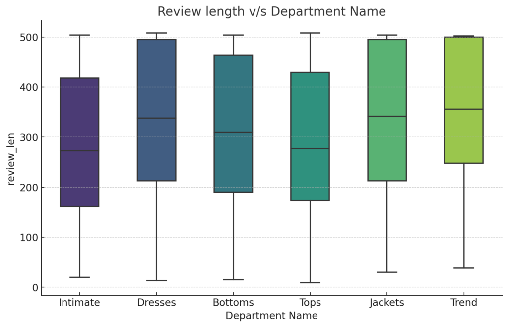
Regarding review length, ‘Jackets’ and ‘Trend’ departments have longer reviews on average, suggesting that customers tend to provide more detailed feedback for these products. The ‘Intimate’ department, while having high ratings, sees shorter reviews, possibly indicating straightforward satisfaction without the need for extended commentary. The tighter interquartile range for ‘Dresses’ and ‘Tops’ suggests that feedback length for these departments is more consistent compared to others.
COMING SOON! HOW TO READ A BOXPLOT VISUALIZATION
Analyzing Reviews Based on Recommendation
To dive deeper into customer feedback, we segmented the reviews based on whether a product was recommended by the user or not. This allows us to glean insights into the sentiment, rating, and length of the feedback.
1. Sentiment Polarity Based on Recommendation
recommended = df.loc[df['Recommended IND'] == 1, 'Polarity']
not_recommended = df.loc[df['Recommended IND'] == 0, 'Polarity']

plt.figure(figsize=(8, 6))
sns.histplot(x=recommended, color=colors[1], label='Recommended')
sns.histplot(x=not_recommended, color=colors[3], label='Not Recommended')
plt.title('Distribution of Sentiment polarity of reviews based on Recommendation', size=15)
plt.legend()
plt.show()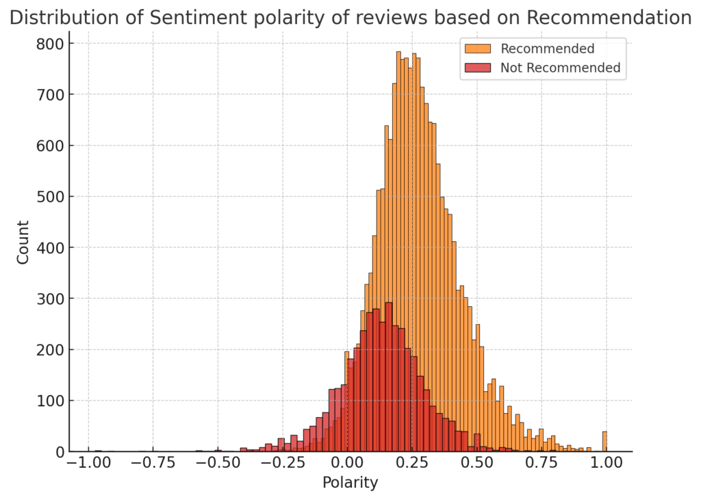
It is observed that reviews that recommend the product tend to have a higher sentiment polarity, indicating a more positive sentiment overall. Also, reviews that do not recommend the product show a wider distribution of sentiment polarities, with a noticeable peak in the negative region, suggesting dissatisfaction.
2. Rating Distribution Based on Recommendation
recommended = df.loc[df['Recommended IND'] == 1, 'Rating']
not_recommended = df.loc[df['Recommended IND'] == 0, 'Rating']

plt.figure(figsize=(8, 6))
sns.distplot(x=recommended, color=colors[1], label='Recommended', )
sns.distplot(x=not_recommended, color=colors[3], label='Not Recommended')
plt.title('Distribution of Rating of reviews based on Recommendation', size=15)
plt.legend()
plt.show()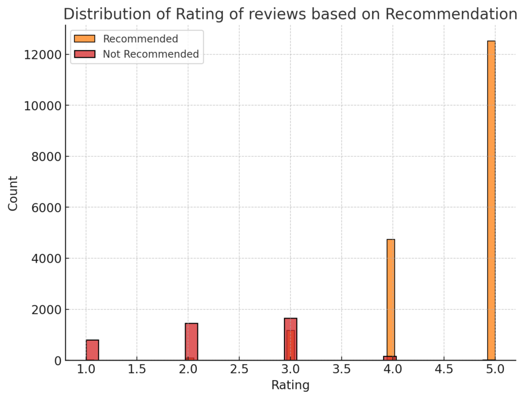
As expected, reviews recommending the product predominantly have higher ratings, especially in the 4 and 5-star categories. While reviews that do not recommend the product show a spread across lower ratings, with notable peaks at 1 and 2 stars.
3. Review length Distribution Based on Recommendation
recommended = df.loc[df['Recommended IND'] == 1, 'review_len']
not_recommended = df.loc[df['Recommended IND'] == 0, 'review_len']

plt.figure(figsize=(8, 6))
sns.histplot(x=recommended, color=colors[1], kde=True, label='Recommended', binwidth=8)
sns.histplot(x=not_recommended, color=colors[3], kde=True, label='Not Recommended', binwidth=8)
plt.title('Distribution of Review length of reviews based on Recommendation', size=15)
plt.legend()
plt.show()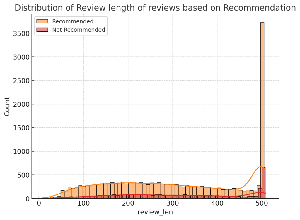
It is observed that both recommended and not-recommended reviews exhibit a broad range of review lengths. Interestingly, reviews that do not recommend the product tend to be slightly longer on average. This could suggest that dissatisfied customers often provide more detailed feedback or explanations for their dissatisfaction.
Exploring Bivariate Distributions: 2D Density Joint Plots
This is also known as Kernel Density Estimation (KDE) joint plots and is an example of bivariate analysis. When analyzing customer reviews, understanding the interplay between different attributes can provide deeper insights into customer behavior and preferences. The 2D Density joint plots, or simply 2D Density plots, help in visualizing the distribution of two variables simultaneously, revealing areas of high and low data concentration, it does this without making any assumptions about the underlying data distribution.
Rating vs. Sentiment Polarity
plt.figure(figsize=(8, 8))
g = sns.jointplot(x='Rating', y='Polarity', kind='kde', color=colors[3], data=df)
g.plot_joint(sns.kdeplot, fill=True, color=colors[3], zorder=0, levels=6)
plt.show()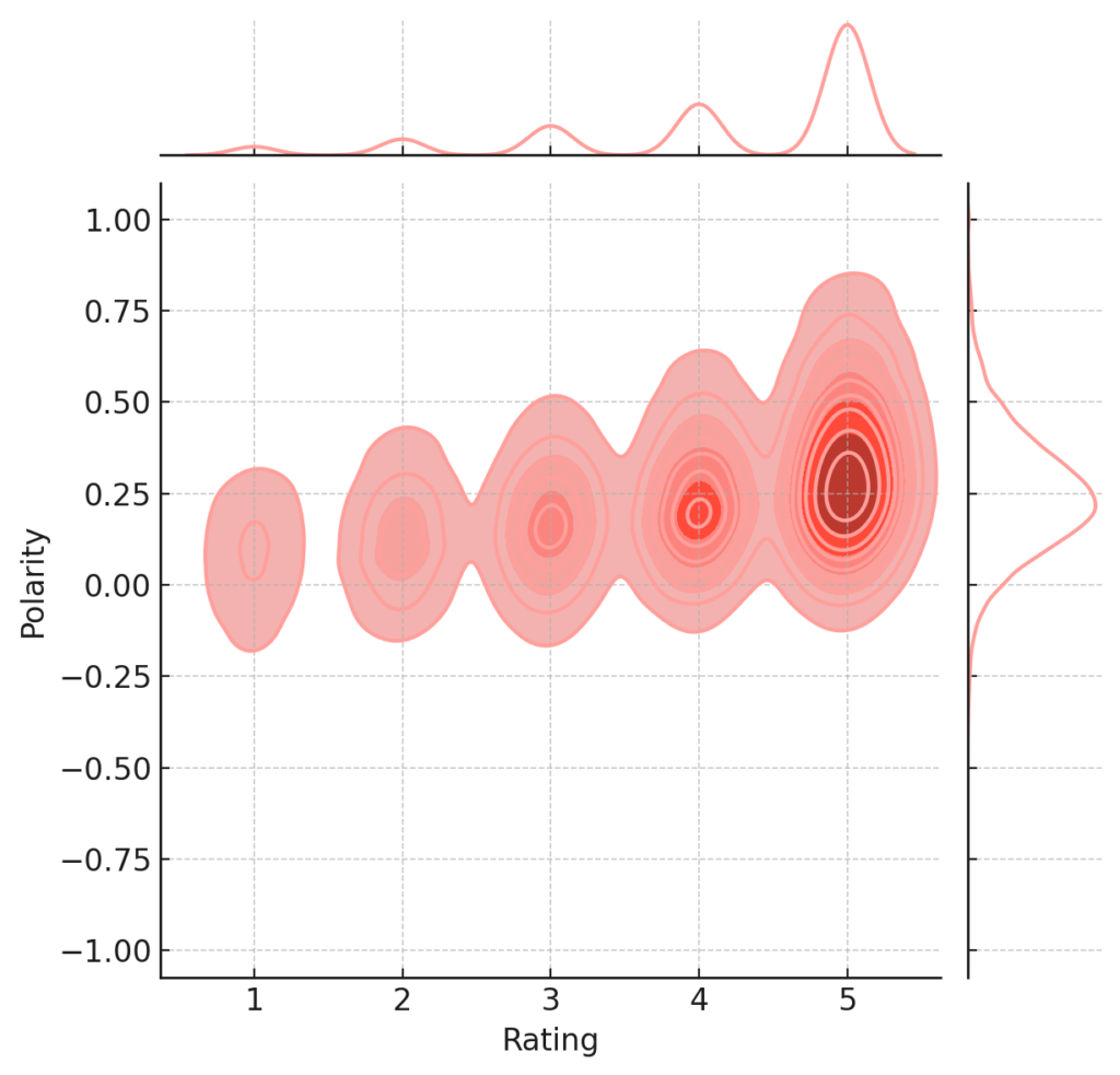
The joint plot between Rating and Polarity illustrates how customer sentiment, as captured by polarity, relates to the numeric rating given. Key observations from the plot:
- Positive Correlation: As expected, higher ratings generally align with more positive sentiments. This is evident from the dense concentration in the upper-right quadrant of the plot.
- Ambiguity in Neutral Polarity: Reviews with a neutral sentiment polarity (around 0) have a wide range of ratings, suggesting that customers might have mixed feelings or the review text might not be explicitly positive or negative.
- Low Ratings with High Negative Polarity: There’s a clear concentration of low ratings with highly negative sentiment. This emphasizes that very negative reviews often come with the lowest ratings.
Age vs. Sentiment Polarity
plt.figure(figsize=(10, 8))
g = sns.jointplot(x='Age', y='Polarity', kind='kde', color=colors[1], data=df)
g.plot_joint(sns.kdeplot, fill=True, color=colors[1], zorder=0, levels=6)
plt.show()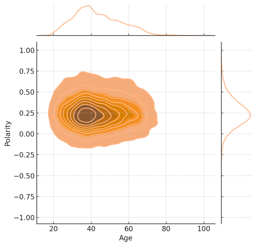
Analyzing the relationship between a customer’s age and the sentiment polarity of their review can offer insights into how different age groups perceive products. Key observations:
- Uniform Sentiment Across Age Groups: There doesn’t seem to be a strong correlation between age and sentiment. People of all ages can have both positive and negative experiences.
- High Concentration in Middle Ages: There’s a noticeable concentration around the middle age groups with neutral to positive sentiment. This might suggest that this age group is more active in leaving reviews or perhaps they have more consistent experiences.
- Sparse Data for Extreme Ages: The plot is less dense at the lower and higher age spectrum, indicating fewer reviews from very young or very old customers.
Conclusion:
Looking through online fashion reviews can be tricky, but with the right tools and methods, businesses can get valuable insights. Our deep dive into e-commerce clothing reviews shows the details of customer feedback, sentiment, and preferences. By using these insights, e-commerce platforms can improve their products and marketing, ensuring a better shopping experience for everyone. As online shopping continues to change, listening to customer feedback will always be important for success.