Introduction
Heart failure is a serious medical condition in which the heart is unable to pump enough blood to meet the body’s needs. It is a leading cause of death worldwide and poses a significant public health challenge. Early detection and accurate prediction of heart failure risk are crucial for timely intervention and effective management of patients.

In recent years, machine learning has emerged as a transformative force in healthcare. By harnessing the power of algorithms that can learn from and make predictions on vast amounts of data, healthcare professionals are now better equipped to diagnose diseases, forecast patient trajectories, and even tailor treatments to individual patients. Specifically, predictive modeling using machine learning can analyze patterns from past medical data to make informed predictions about future health outcomes. This not only enhances the accuracy and speed of diagnoses but also paves the way for personalized medicine, where treatment plans are customized to each patient’s unique profile. In this context, our endeavor to predict heart failure using machine learning showcases the potential of such techniques in addressing critical health challenges.
Background Information
Heart failure occurs when the heart becomes weakened or damaged, resulting in a reduced ability to pump blood effectively. It can be caused by various factors, including coronary artery disease, hypertension, heart valve disorders, and cardiomyopathy. Identifying the risk factors and early signs of heart failure can significantly improve patient outcomes and reduce mortality rates.
The advent of electronic health records (EHRs) has revolutionized modern healthcare. These comprehensive digital repositories store a patient’s medical history, diagnoses, medications, treatment plans, immunization dates, allergies, and even radiology images. Beyond just digitizing patient information, EHRs play a pivotal role in data-driven healthcare, offering a wealth of data ready for analysis.
Coupled with the advancements in machine learning, EHRs have unlocked unprecedented possibilities in predictive healthcare modeling. Machine learning algorithms, with their ability to sift through vast datasets and identify intricate patterns, can extract meaningful insights from EHRs that might elude traditional analyses. This synergy between EHRs and machine learning is particularly promising for conditions like heart failure, where early prediction can make a significant difference in patient outcomes. Our project taps into this potential, leveraging historical patient data to predict heart failure risks.
Dataset Overview
The dataset used for this project contains various clinical and demographic features of patients, along with a binary target variable indicating whether they experienced a heart failure event or not. Here’s a comprehensive list of the features:
- age: The age of the patient (numeric).
- anaemia: Whether the patient has anemia or not (0 = No, 1 = Yes).
- creatinine_phosphokinase: Level of creatinine phosphokinase enzyme in the blood (numeric).
- diabetes: Whether the patient has diabetes or not (0 = No, 1 = Yes).
- ejection_fraction: Percentage of blood leaving the heart at each contraction (numeric).
- high_blood_pressure: Whether the patient has hypertension or not (0 = No, 1 = Yes).
- platelets: Platelet count in the blood (numeric).
- serum_creatinine: Level of serum creatinine in the blood (numeric).
- serum_sodium: Level of serum sodium in the blood (numeric).
- sex: Gender of the patient (0 = Female, 1 = Male).
- smoking: Whether the patient smokes or not (0 = No, 1 = Yes).
- time: Follow-up period in days (numeric).
- DEATH_EVENT: Binary target variable (0: No heart failure event, 1: Heart failure event).
Each row of the dataset represents a unique patient, with their corresponding clinical and demographic details. The “DEATH_EVENT” column indicates whether they experienced a heart failure event during the observation period.
The objective is to use this dataset to develop a predictive model that can accurately classify patients as high-risk or low-risk for heart failure based on their medical characteristics. This will help healthcare professionals in early intervention, personalized treatment, and improving overall patient care.
IMPLEMENTATION
The full code + dataset can be assessed here
Step 1. Importing Libraries and Data
The code begins by importing the necessary Python libraries for data manipulation and visualization. These libraries include NumPy, Pandas, Matplotlib, Seaborn, Scikit-learn, and Keras.
import warnings
warnings.filterwarnings('ignore')

import numpy as np
import pandas as pd
import matplotlib.pyplot as plt
import seaborn as sns
from sklearn import preprocessing
from sklearn.preprocessing import StandardScaler
from sklearn.model_selection import train_test_split

from sklearn import svm
from keras.layers import Dense, BatchNormalization, Dropout, LSTM
from keras.models import Sequential
from keras import callbacks
from sklearn.metrics import precision_score, recall_score, confusion_matrix, classification_report, accuracy_score, f1_score
2. Data Exploration
After importing the required libraries, the code loads the heart failure dataset using Pandas’ read_csv() function. It then proceeds to examine the first few rows of the dataset to get a quick glimpse of what the data looks like using the head() function. Additionally, it checks the data types of each column and identifies any missing values using the info() function.
#loading data
data_df = pd.read_csv("data.csv")
data_df.head()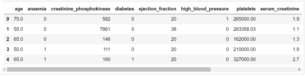
3. Data Visualization
Next, the code performs data visualization to gain insights into the dataset. It starts by visualizing the distribution of the target variable “DEATH_EVENT” using a count plot. This plot helps us understand the balance of the classes in the target variable, which is essential for predicting heart failure outcomes.
cols= ["#CD5C5C","#FF0000"]
ax = sns.countplot(x= data_df["DEATH_EVENT"], palette= cols)
ax.bar_label(ax.containers[0])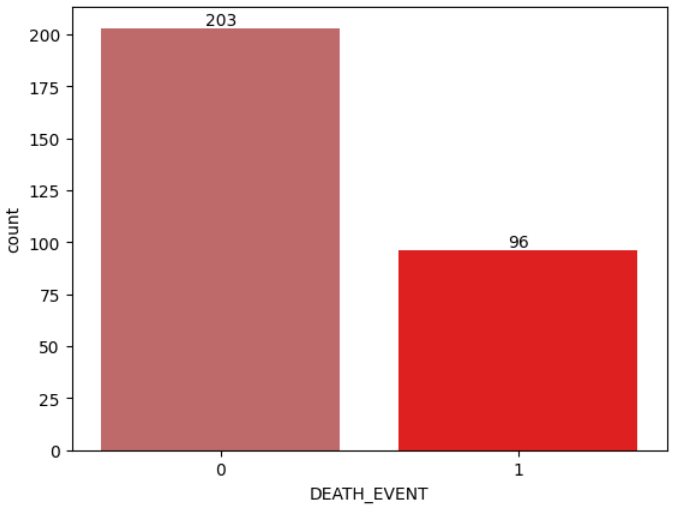
4. Descriptive Statistics and Correlation Analysis
The code then calculates descriptive statistics (like mean, standard deviation, etc.) of the numerical features in the dataset using the describe() function. This helps in understanding the central tendencies and spread of the data.
data_df.describe().T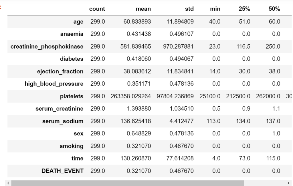
After that, it creates a correlation matrix to visualize the relationships between different features using a heatmap. The heatmap uses colors to represent the strength and direction of correlations between features. It helps in identifying which features are strongly correlated with each other, which can be valuable for feature selection.
cmap = sns.diverging_palette(2, 165, s=80, l=55, n=9)
corrmat = data_df.corr()
plt.subplots(figsize=(20,20))
sns.heatmap(corrmat,cmap= cmap,annot=True, square=True)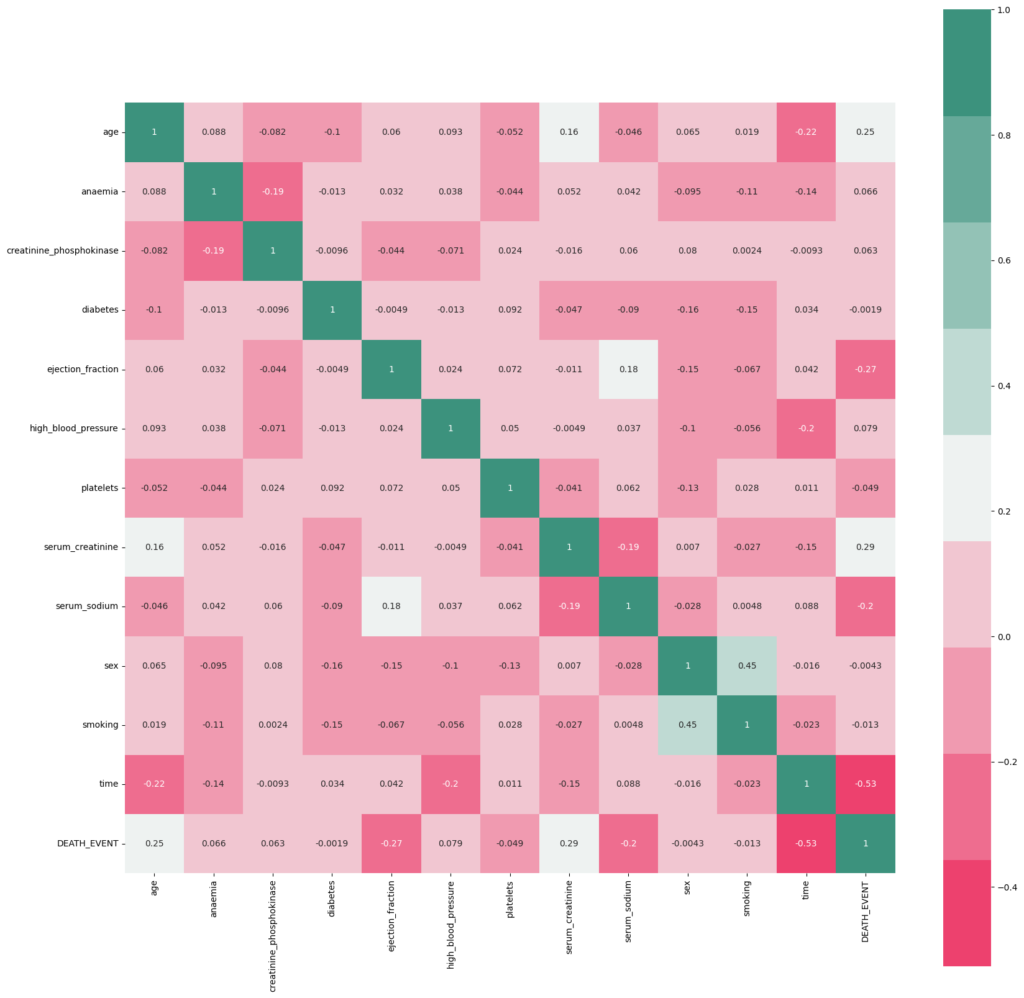
5. Data Preprocessing
Before training the machine learning models, the code prepares the data for modeling. It separates the features (X) from the target variable (y). The features are all the columns in the dataset except for the “DEATH_EVENT” column, which is the target variable we want to predict.
Then, it standardizes the numerical features using Scikit-learn’s StandardScaler. Standardization scales the data to have a mean of zero and a standard deviation of one, which is a common practice in machine learning to ensure all features are on the same scale.
# Defining independent and dependent attributes in training and test sets
X=data_df.drop(["DEATH_EVENT"],axis=1)
y=data_df["DEATH_EVENT"]

# Setting up a standard scaler for the features and analyzing it thereafter
col_names = list(X.columns)
s_scaler = preprocessing.StandardScaler()
X_scaled= s_scaler.fit_transform(X)
X_scaled = pd.DataFrame(X_scaled, columns=col_names)
6. Further Data Visualization
The code visualizes the scaled numerical features using boxen plots. Boxen plots show the distribution of each feature’s data points, helping to identify any potential outliers and gain a better understanding of their distributions.
#Plotting the scaled features using boxen plots
colors =["#CD5C5C","#F08080","#FA8072","#E9967A","#FFA07A"]
plt.figure(figsize=(20,10))
sns.boxenplot(data = X_scaled,palette = colors)
plt.xticks(rotation=60)
plt.show()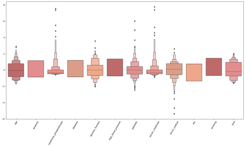
7. Train-Test Split
To evaluate the model’s performance, the dataset is divided into training and testing sets using Scikit-learn’s train_test_split() function. The model will be trained on the training set and evaluated on the test set, ensuring that the model’s generalization ability is tested on unseen data.
#spliting variables into training and test sets
X_train, X_test, y_train,y_test = train_test_split(X_scaled,y,test_size=0.30,random_state=25)
8. Model 1: Support Vector Machine (SVM)
The code initializes an SVM model using Scikit-learn’s SVC class. SVM is a machine learning algorithm used for classification tasks. It then fits the SVM model to the training data using the fit() method, which means it trains the model to learn patterns from the training data.
Next, the code makes predictions on the test data using the predict() method of the SVM model. These predictions are compared to the actual labels of the test data to evaluate the model’s performance.
# Instantiating the SVM algorithm
model1=svm.SVC()

# Fitting the model
model1.fit (X_train, y_train)

# Predicting the test variables
y_pred = model1.predict(X_test)

# Getting the score
model1.score (X_test, y_test)
9. Model 2: Artificial Neural Network (ANN)
The code constructs an artificial neural network using the Keras library, which is a popular deep learning framework in Python. Here’s a breakdown of the model’s architecture and training process:
Early Stopping: To prevent overfitting and optimize training time, an early stopping callback is utilized. It monitors the model’s performance and stops the training process if there’s no significant improvement observed (defined by a minimum delta) for 20 consecutive epochs. The best weights during the training are restored to ensure the model’s optimal performance.
Model Initialization: The neural network model is initialized using the Sequential class, which allows the stacking of layers linearly.
Input Layer: The first layer has 16 neurons, uses the relu activation function, and expects 12 input features, matching the number of features in our dataset.
Hidden Layers:
The second layer consists of 8 neurons with relu activation.
A dropout layer follows it with a rate of 0.25, randomly setting a fraction of the input units to 0 during training, which helps prevent overfitting.
Another dense layer with 8 neurons and relu activation is added.
This is followed by another dropout layer, but with a higher rate of 0.5.
Output Layer: The final layer has a single neuron with a sigmoid activation function. Since this is a binary classification problem, the sigmoid activation ensures the output is between 0 and 1, representing the probability of the positive class.
Model Compilation: The model is compiled using the adam optimizer and the binary_crossentropy loss function, which is suitable for binary classification tasks. The metric used to evaluate the model’s performance during training is accuracy.
Model Training: The ANN is trained using the fit method on the training data. The batch size is set to 25, and the model trains for a maximum of 80 epochs. However, the training may stop early due to the early stopping callback. During training, 25% of the training data is set aside as a validation set to monitor the model’s performance on unseen data. Below is the code snippet for this section.
early_stopping = callbacks.EarlyStopping(
    min_delta=0.001, # minimium amount of change to count as an improvement
    patience=20, # how many epochs to wait before stopping
    restore_best_weights=True)

# Initialising the NN
model = Sequential()

# layers
model.add(Dense(units = 16, kernel_initializer = 'uniform', activation = 'relu', input_dim = 12))
model.add(Dense(units = 8, kernel_initializer = 'uniform', activation = 'relu'))
model.add(Dropout(0.25))
model.add(Dense(units = 8, kernel_initializer = 'uniform', activation = 'relu'))
model.add(Dropout(0.5))
model.add(Dense(units = 1, kernel_initializer = 'uniform', activation = 'sigmoid'))

# Compiling the ANN
model.compile(optimizer = 'adam', loss = 'binary_crossentropy', metrics = ['accuracy'])

# Train the ANN
history = model.fit(X_train, y_train, batch_size = 25, epochs = 80,callbacks=[early_stopping], validation_split=0.25)
10. Model Evaluation
The code calculates and prints various evaluation metrics such as accuracy, precision, recall, F1-score, and a confusion matrix to assess how well the SVM model is performing in predicting heart failure outcomes.
SUMMARY
Heart failure, a condition where the heart can’t pump blood efficiently to meet the body’s needs, remains a leading cause of mortality globally. Early detection and precise prediction of heart failure risk are paramount for timely interventions and tailored patient management. Addressing this critical healthcare challenge, this project harnesses the power of machine learning to analyze clinical and demographic data, aiming to identify individuals more susceptible to heart failure. Through the utilization of advanced algorithms and comprehensive data analysis techniques, the developed model seeks to empower healthcare professionals with predictive insights, facilitating early intervention and enhancing patient care outcomes.
Proposed future work
The prediction of heart failure is recognized as a crucial task with significant implications for healthcare. For the enhancement of the heart failure prediction model and its broader usability, the following steps for future work are proposed:
- Data Collection and Enhancement:
- Diverse and extensive datasets from varied sources and demographics are to be collected, aiming to bolster the model’s generalization capabilities.
- Additional relevant features, such as lifestyle habits, medical history, and genetic factors, are to be explored for their potential insights into heart failure prediction.
- Feature Engineering:
- In-depth feature engineering is to be conducted, creating or transforming features to better represent underlying data patterns.
- Domain knowledge and medical expertise are to be leveraged to derive meaningful information from the raw data.
- Handling Imbalanced Data:
- The issue of imbalanced classes in the target variable is to be addressed using techniques like oversampling, undersampling, or synthetic data generation.
- Advanced resampling methods like SMOTE are to be employed for the creation of synthetic examples.
- Advanced Modeling Techniques:
- More advanced machine learning algorithms and ensembles, such as Random Forests, Gradient Boosting Machines, and XGBoost, are to be explored.
- Deep learning architectures, like RNNs or LSTMs, are to be investigated for their potential in capturing sequential patterns.
- Hyperparameter Tuning:
- Optimization of machine learning models’ hyperparameters is to be performed using methods like grid search or random search.
- Interpretability and Explainability:
- Techniques for interpreting and explaining the model’s predictions are to be implemented, aiding medical professionals in understanding the decision-making process.
- Cross-Validation and Performance Metrics:
- K-fold cross-validation is to be employed for a reliable estimation of model performance.
- Consideration is to be given to additional healthcare-specific performance metrics such as sensitivity, specificity, and AUC-ROC.
- Deployment and Integration:
- A user-friendly web application or interface is to be developed, allowing easy access for medical professionals.
- Integration with electronic health record systems is to be facilitated for real-time prediction capabilities.
The full Code implementation and dataset used can be assessed here
Reach out to me via email (vokallond@gmail.com) if you want to learn machine learning from scratch